Vista Alignment Tools |
||||||||||||||||||||||||
The Vista Point suite of tools provides an integrated set of resources for visualizing and
exploring Vista DNA alignments. This toolkit allows you to switch among
three visualization modes for examining the same alignment:
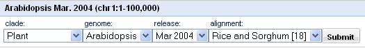
1. VistaPoint1.1. OverviewThe application enables visual comparative analysis of complete genome assemblies at different levels of resolution, using pairwise and multiple large-scale alignments. A visual representation of the alignments is comprised of two parts: graphs panel and alignments table, which are described in detail below. 1.2. Genome SelectionAnalysis begins with the selection of a base genome and a compared genome from the pull-down menus shown in Figure 1.
1.3. NavigationUse the controls located on the Chromosome Panel (Figure 2).
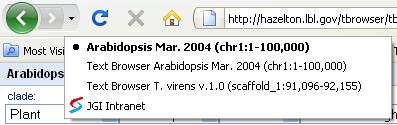
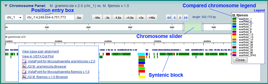
The navigation buttons along with the chromosome slider allow for zooming and panning along the interval of the base chromosome. The slider region represents the entire base chromosome/scaffold, while the "thumb" (the greenish area) represents the region currently displayed in the panel above. The displayed region can be specified explicitly by entering it into the position box and clicking Go. Alternatively, you can enter a part of a gene symbol or name, in which case you will be prompted to choose from the list of genes that contain this pattern as part of their symbols or names. The displayed region can also be changed by sliding or resizing the thumb (grabbing and dragging its edge). The history support is leveraged by the location bar history of a web browser, allowing you to go back to the previous view, or forward to the next view in history, as well as to jump back or forward over the several views (Figure 3).
1.4. Graphs panel1.4.1. AnnotationThe gene annotation track is shown above the conservation curves, where dark and light blue boxes represent exons and UTRs respectively. Gene name appears underneath the track, the arrow points in the direction of the gene. (Figure 4).
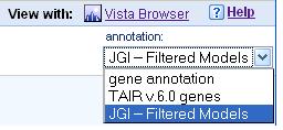
Some genomes may have multiple annotations available. In this case you can display different annotations by selecting them from the "annotation" list box (Figure 5).
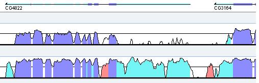
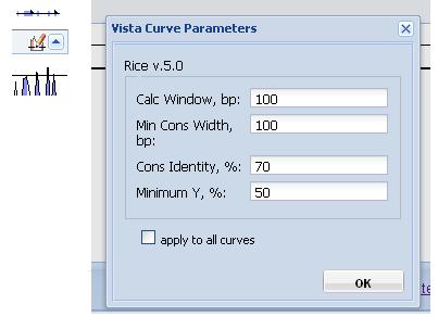
1.4.2. Peaks and valleys.The VISTA curve is calculated as a windowed-average identity score for the alignment. Each "peaks and valleys" graph represents percent conservation between aligned sequences at a given coordinate on the base genome according to the following: 1.4.3. Colored conserved regions. Regions are classified as "conserved" by analyzing scores for each base pair in the genomic interval, that is "Minimum Conserved Width" (default value 100 bp) and "Conservation Identity" (default value 70%). A region is considered conserved if the conservation over this region is greater than or equal to the "Conservation Identity" and has the minimum length of "Minimum Conserved Width". Regions of high conservation are colored according to the annotation as exons (dark blue), UTRs (light blue) or non-coding (pink). The thresholds that determine what gets colored, as well as minimum and maximum percentage bounds can be adjusted as the following: 1.4.4. Changing curve parameters.To adjust the parameters for a particular curve, click the "Vista Curve Parameters" button, a form with the adjustable parameters will appear (Figure 6).
Calc Window: The size of the sliding window used to calculate the conservation scores of each base pair used in the calculation of VISTA curve. Default is 100 base pairs. Min Cons Width: Minimum width a conserved region must be before it is painted as such. Default value is 100 base pairs. Cons Identity: Minimum percent conservation identity that must be maintained over the window ("Min Cons Width") for a region to be considered conserved. Default value is 70%. Minimum Y: Lower boundary of the graph. Dropping the minimum Y value in areas of low conservation will allow you to see the smaller peaks. Default value is 50%. 1.4.5. Changing the order of curves.To change the order in which the curves are displayed on the panel, position the mouse cursor over the curve title (the cursor will be changed as an indication that the dragging is enable), and drag the curve to the new position. 1.4.6. Zooming.To zoom in, click one of the "zoom in" buttons (+1.5x, +3x, +10x), located on the Chromosome Panel, or highlight the area of the graph you want to see in detail by holding down the left mouse button while moving the mouse over the region of interest, just like you would highlight a sentence in Word. The browser will zoom in on the selected area once you let go of the mouse button. 1.5. Alignments tableThe table is located inside a resizable, collapsible panel, a panel's header contains a link to download a selected gene annotation of a base genome, and a link to a list of all conserved regions found (Figure 7).
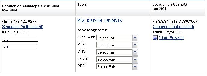
The table lists each alignment that was generated for the base organism. Each row is a separate alignment. Each column, except the Tools, refers to the genome sequence that participates in a run. The Tools column contains information pertaining to the whole alignment (Figure 8).
The first cell of each row also contains a preview of the Vista plot of this particular alignment, which allows one to quickly evaluate the quality of this alignment and to see alignment overlaps. Tools column provides links to alignments in human readable and MFA (multi-fasta alignment) formats, a list of conserved regions from this alignment alone (CNS), and links to PDF plots of this alignment alone. If the region being examined is 20K or less, rVista analysis can be performed, and a link to rVista will also be displayed here. This column also provides links to results of rankVista analyisis of the alignment. Read more about RankVista here. By looking at a row in this table, you can see which section of each organism aligned to which. The Sequence links will return a fasta-formatted piece of the organism sequence that participates in the alignment. Clicking on the Vista Browser links will launch the applet with the corresponding organism selected as base, and the coordinates set to the coordinate of the selected alignment. Detailed help and instructions on the applet are available here. The PDF file stores the visual representation of the alignment and found conserved regions, conservation and annotation coloring rules are similar to the graph panel described above. Gaps in the base sequence are signified by red sections of line underneath the plot. The color legend is summarized in the upper left-hand corner of the display. The gray lines under the plot show contigs, which are numbered in the case of draft sequences. 2. The Vista Synteny ViewerThe Vista Synteny Viewer application enables pair-wise comparative analysis of genome assemblies at three levels of resolution. Its use is described below: 2.1. Genome SelectionAnalysis begins with the selection of a reference genome and a compared genome from the pull-down menus shown in Figure 1.
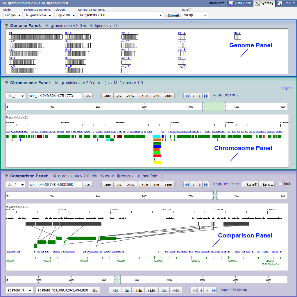
The cutoff defines the minimal length for inclusion of an alignment in the analysis. 2.2. The Synteny Viewer2.2.1 Overview of the Synteny BrowserThe Synteny Browser enables visual comparative analysis of complete genome assemblies at different levels of resolution, ranging from genome-scale comparison of chromosomes to comparisons of individual regions of alignment at the nucleotide level. Synteny in the Synteny Browser is calculated referenced on pair-wise whole genome alignment. Genomic synteny is displayed in three collapsible panels in the Synteny Browser: the Genome Panel, the Chromosome Panel and the Compared Panel (Figure 2) .
Each of the panels in the Synteny Browser can be collapsed or expanded in order to preserve vertical space on the page. To collapse or expand a panel, click on panel's title bar. 2.2.2. The Genome Panel
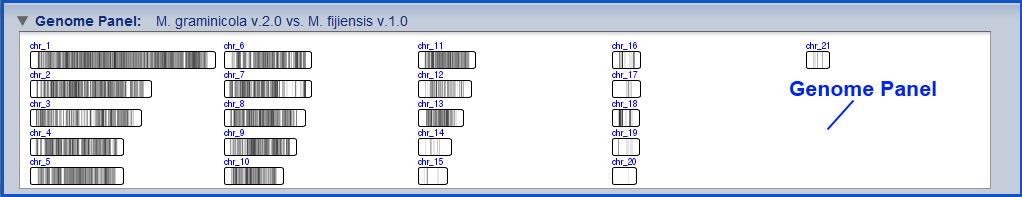
The Genome Panel (Figure 3) shows the chromosomes of the reference genome, colored to indicate alignment density. Here, alignment density is defined for a region in the reference genome as the number of regions in the compared genome to which it has synteny. Darker regions in the image have higher density of coverage. Clicking on a chromosome in The Genome Panel displays a region of this chromosome in the Chromosome panel. 2.2.3. The Chromosome PanelThe Chromosome panel (Figure 4) displays synteny between a given interval on a reference-genome chromosome and the entire compared genome.
Synteny is depicted as "blocks" along the reference-genome interval. Each block represents an alignment of two sequences, where the position of the block indicates the alignment's location on the reference genome and the color of the block indicates the chromosome where the match is found on the compared genome. Click on Legend to reveal the color-coding schema. The blocks appear stacked on top of each other when a fragment of the reference genome has synteny with multiple locations in the compared genome. The navigation buttons along with the chromosome slider allow for zooming and panning along the interval of the reference chromosome. The slider area represents the entire reference chromosome/scaffold, while the "thumb" (the pink box) represents the region currently displayed in the panel below. The displayed region can be changed by sliding or resizing the thumb (grabbing and dragging its edge). The displayed region can also be specified explicitly by entering it into the position box and clicking Go. Syntenic blocks are interactive. Clicking on a block displays the alignment at higher resolution in the Compared Panel (see below). Hovering the mouse over a block brings up a pull-down context menu which allows the user to display these regions in other browsers or to see the base-pair alignment corresponding to the block. Figure 4 show a view of the Chromosome panel with this context menu opened for a moused-over syntenic block. When available for a given genome, a Gene model track will appear between the slider and the synteny blocks. Predicted gene models appear as black lines with exonic regions indicated by purple blocks. An arrow on either the right (forward) or left (reverse )end of the gene model indicates the strandedness of the gene. Clicking on a gene will take you to the protein page, if available, for the given gene model on the website that provided the prediction (e.g. usually a JGI Genome Portal protein page). 2.2.4. The Comparison PanelThe Compared Panel displays the alignment between specific regions on both the reference and compared genomes (Figure 5).
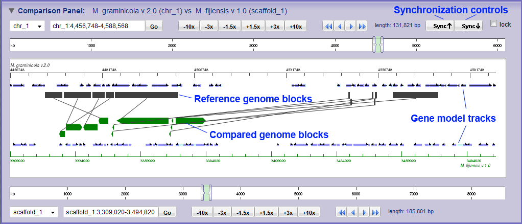
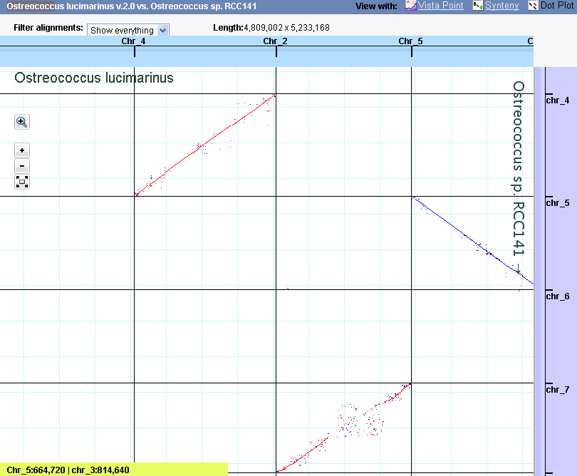
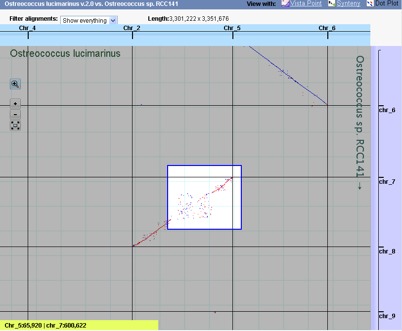
In this view, each aligned region is depicted as a pair of blocks, one along the reference chromosome (grey) and one along the compared chromosomes (colored), connected by a line. Also displayed in the Compared Panel are gene model tracks (if available) for the reference and compared chromosomes. Syntenic blocks and gene models are both interactive, as described above for the Chromosome Panel. Navigation controls allow the user to switch chromosomes, zoom and pan independently over the reference and compared genomes. The Chromosome Panel and Comparison Panel can be navigated independently and may display different regions of the reference genome. The Sync Up and Sync Down buttons allow the user to synchronize these two views to match the reference region displayed in the Compared Panel or Chromosome Panel, respectively. If Lock is checked, this synchronization is maintained as the user navigates the reference genome region in either Panel. 3. VistaDotVistaDot (Figure 1) is an interactive tool that enables users to look at the DNA conservation between two genome assemblies at different levels of resolution and across multiple chromosomes/scaffolds.
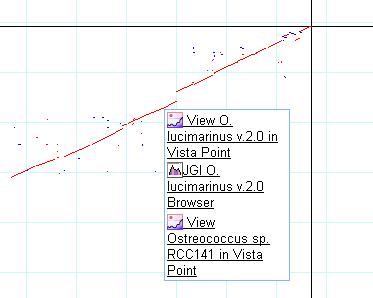
In the main view window DNA coordinates of the reference genome are presented on the X axis, and DNA coordinates of the compared genome are presented on the Y axis. All chromosomes or scaffolds are concatenated together, usually in a descending order by size. The diagonal lines in the image display the homologous regions between the two genomes. If the line is blue, the regions are on the same strand. If the line is red, the regions are on opposite strands. The grid in black lines indicates scaffold/chromosome boundaries. A cutoff control above the main window allows you to Filter alignments to show only syntenic regions greater than a specified length. Next to the cutoff control, the Length of the region currently on-screen is shown (length of x-axis genome, length of y-asix genome). As you move the mouse across the main windown, the Genome coordinates of current cursor position are shown in the yellow box at the bottom left of the view. The first set of coordinates corresponds to reference genome and the second set of coordinates refers to the compared genome. Linking out from a segment of the alignment
Dot plot NavigationYou can pan and zoom within the Dot Plot in a variety of ways:
Gene tracks in Dot PlotWhen you zoom on either axis to a region of length < 200kb, gene model predictions will appear along the edge of the main window (Figure 4). Red boxes indicate gene models predicted on the forward strand, while blue boxes indicate genes on the reverse strand. If you hover the mouse over a gene you will see the gene model name. Note: Gene tracks are not available for all genomes.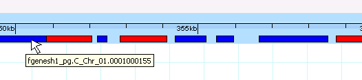 Figure 4: The Gene Track |