Using VISTA Browser

VISTA Browser requires Java 1.2 or better. If you experience problems such as a gray screen with no browser, an empty window, etc. you need to install Java. Please follow the instructions below to install it. If you have any problems with the installation process or with the browser, and they are not addressed in these help pages, please contact us at vista@lbl.gov. We welcome all feedback.

We do not currently support Java 1.5. Some features of the browser may not work properly if you have this version of Java installed on your computer.

1. Installing Java
2. Overview
3. Navigation
   1. Understanding the display
      (Peaks and Valleys, Annotation, Colored Regions, Contigs)
   2. RankVISTA
   3. How to navigate the browser
      (Position control, Gene Search, Changing annotations, Adding and Removing Curves, Scrolling and Zooming, Browsing History)
   4. Nucleotide level alignment panel
4. Utilities
   1. Printing
   2. Saving
   3. Retrieving alignments
   4. Retrieving annotations
   5. Retrieving sequences
   6. Submitting to rVista
   7. Viewing in other Browsers
5. Advanced
   1. Changing the base genome
   2. How the curve is calculated
   3. Changing curve parameters
   4. Changing the number of rows
   5. Changing the order of Curves
   6. Overlapped contigs
   7. Coloring Rules
6. Troubleshooting
   1. Browser and Information buttons don't work!
   2. Browser does not print from Opera

-Click any of the Figures for a larger version-

Installing Java

Follow these instructions to install Java on your machine:
Windows | Linux | Solaris

We have found that the latest Java release, Java 1.5, has some bugs that prevent certain features, most notably printing, from working properly. We urge users not to upgrade to 1.5 just yet, and wait until those issues are addressed by Sun. Our instructions tell you how to install the more stable 1.4.2 instead.

If despite the above warning you prefer to install the latest Java version, you can go to http://www.java.com/, click the "Download now" button, and follow the intructions on that page.

Macintosh users should upgrade their OS to 10.1 or better. Additional java upgrades may be available from Apple's download page.

Overview

Vista Browser is an interactive Java applet designed to visualize multiple large-scale alignments. The browser's clean display makes it easy to identify regions of high conservation across multiple species. The browser is used to visualize pairwise and multiple whole genome alignments produced internally as well as alignments produced for GenomeVISTA users who submit their own sequences to be aligned to base genomes such as human, mouse, rat, drosophila, etc.

Navigation

Understanding the display

Fig. 1. VISTA Browser

Fig. 2. Curve Names

Fig. 3. Annotations

Fig. 4. Vista Curves and Contigs

Fig. 5. A sample rankVISTA graph.

Fig. 6. A sample of rankVISTA regions.

Fig. 1 shows a sample screenshot of the VISTA Browser. The browser is divided into three panels: the standard VISTA graph display, the position control panel on the left, and the toolbar.

VISTA graph display

Peaks and Valleys

The "peaks and valleys" graphs represent percent conservation between aligned sequences at a given coordinate on the base sequence (see how the curves are calculated). Multiple alignments that share the base sequence can be displayed simultaneously, one under another. The top and bottom percentage bounds are shown to the right of every row. These bounds can be adjusted (see how to adjust curve settings). The graphs are numbered, so that you can identify each graph in the list underneath the VISTA panel (Fig. 2).

Annotation

The browser shows base genome annotation directly above the curves (Fig. 3). Arrows signifying genes are drawn above the graphs, pointing in the direction of the gene. All exons and UTRs are marked with the same colors as on the VISTA graph. Gene names appear underneath the arrows if there is enough room. Repeats are shown below the genes, colored according to the legend in the lower left-hand corner of the display. SNPs, if they exist, are shown directly above the graphs. This track contains dbSNP, available from ftp.ncbi.nih.gov/snp. When viewing the track at or near base-level resolution, the displayed width of the SNP corresponds to the width of the variant in the reference sequence. On a large region the darkness of a SNP mark corresponds to the SNPs density on this region. SNPs are also indicated on base-pair level alignment panel.

Colored Regions

Regions of high conservation are colored according to the annotation as exons (dark blue), UTRs (light blue) or non-coding (pink) (Fig. 4). The thresholds that determine what gets colored, as well as minimum and maximum Y-axis values, can be easily adjusted (see how to adjust curve settings).

Contigs

The thick gray or red lines under the plot show contigs of the species aligned to the base genome (Fig. 4). The names of these contigs can be seen on the information panel by hovering the mouse cursor over the graph. If the lines are red instead of gray, multiple regions from the second sequence were aligned to this base sequence location, and several alignments are overlapped here (read about overlaps).

RankVISTA display

RankVISTA conservation plots depict evolutionarily conserved segments in pairwise or multiple alignments as a bar graph, where the heights scale with statistical significance [-log₁₀(P-value)]. For example, a height of 4 indicates that the probability of seeing that level of conservation by chance in a neutrally-evolving 10-kb segment of the base sequence is less than 10^-4.

RankVISTA graphs are based on the Gumby algorithm, which estimates neutral evolutionary rates from non-exonic regions in the multiple sequence alignment, and then identifies statistically significant local segments of any length in the alignment that evolve more slowly than the background. The phylogenetically weighted log-odds conservation scores of conserved segments are translated into P-values using Karlin-Altschul statistics. Gumby has no window-size parameter, and no fixed percent-identity threshold. Since the algorithm uses a more-conserved-than background paradigm, it can perform phylogenetic shadowing (close species) and footprinting (distant species) with equal facility.

Note that short functional elements may not be detected as statistically significant in comparisons of very close species. An extreme example: since the human and chimpanzee genomes are 98.7% identical even in neutral regions, the vast majority of exons are too short to stand out as statistically significant in a human-chimpanzee comparison. In general, statistical power to detect short constrained functional elements increases as the total neutral divergence of the compared species increases.

Note: Since the input alignment is its own training set, small or grossly incomplete alignments are to be avoided:

• The base sequence length should be at least 10 kb. Smaller alignments might be tolerated, but if Gumby detects an inadequate number of aligned positions, it will return no output.
• For the p-values to be meaningful, Gumby requires a reasonably complete alignment. Rule of thumb: the number of "N" characters and spurious gap characters arising from missing sequence data should be less than 10% of the total number of characters in the alignment. The relative ranking of conserved regions by pvalue would still be meaningful if this rule were violated. However, the p-value estimates would be systematically biased.
• Gumby's sensitivity in detecting non-exonic conservation can be increased by supplying exon annotations. The annotated regions are masked when estimating neutral evolutionary rates, resulting in a more accurate estimate of the background conservation level.

RankVista regions are colored according to their annotation, as seen in Fig. 5. Note that RankVista coloring is based on exon annotations of all aligned sequences, not just the one currently used as the base. Consequently, an unannotated region in the base sequence might still be colored as an exon because of annotations from other sequences. In another deviation from the standard scheme, RankVISTA colors UTRs and coding exons the same, since they are treated identically by Gumby.

For more information, and to download Gumby source code, please go to http://pga.lbl.gov/gumby

References (the first publication below is the primary reference for Gumby):

Shyam Prabhakar, Francis Poulin, Malak Shoukry, Veena Afzal, Edward M. Rubin, Olivier Couronne, Len A. Pennacchio. Close sequence comparisons are sufficient to identify human cis-regulatory elements. Genome Res. 2006;16(7):855-63.

Qian-fei Wang, Shyam Prabhakar, Sumita Chanan, Jan-Fang Cheng, Edward M. Rubin, Dario Boffelli. Detection of weakly conserved ancestral mammalian regulatory sequences by primate comparisons. Genome Biology 2007;8(1):R1.

How to Navigate the Browser

Fig. 7. Control Panel

The left panel of the browser is divided into three parts: Control Panel, Information, and the Legend.

Gene Search

The Control Panel (Fig. 7) features a drop-down box called "Reference (Base) genome," which lists all available base genomes. The current one is selected. Changing the base genome in this box will switch over the whole browser; the current curves and annotations will disappear, and the browser will go to the default location on the newly selected genome (see adding curves for more information).

Position Control Panel

The next field specifies the genome segment displayed by the Browser. To change positions, one can enter specific coordinates on the genome, such as chr9:102,923,121-103,070,274 or contig1080:11152-7781, a gene name, or a contig name. Press the "enter" key. The browser will go directly to the location of the gene if there is only one exact match, or display a dialog box if there are more than one. Partial gene names are accepted. Please note that the browser does have an upper limit on the size of the region it can display at a time. At this time, it is slightly above 5 million base pairs.

Changing annotations

Some genomes may have multiple annotations available. If you wish to change the annotation you are viewing, you can do so by using the "Gene Annotation" menu in the left-hand panel, directly below the "Position" field.

Adding and Removing Curves

To add a curve, make sure that the correct base genome is selected in the "Base (Reference) Genome" menu (please note that changing the base genome will result in switching to that genome, getting rid of any curves that are on the screen at the moment). Use the drop-down menu to select and add a new organism. The counter above the drop-down menu shows how many organisms are available in addition to the ones currently displayed on the screen.

Alternatively, you can click the "add curve" button. You will see the "Add New Curve" dialog box. In most cases, selecting the data set you want to see aligned to the base genome is sufficient - just fund it in the drop-down list, and click "ok". If you wish, you can change parameters used to calculate the curve and conserved regions, and change the minimum and maximum y-axis values. You can also edit the curve name that describes this curve (this is most useful if you wish to look at two alignments of the same genomes with different calculation parameters).

The two items in the Information Panel, Position and Contig, show information about the position on the graph that the mouse is hovering over. Position displays the exact base genome coordinate, and Contig shows the name of the corresponding contig on the mapped data set.

Scrolling and Zooming

In addition to navigating the browser by entering exact coordinates in the position control panel and searching by gene names, the browser provides all the standard scrolling and zooming functions. To move left or right by half the size of the current region, click the "scroll left/right" buttons. To zoom in, click the "zoom in" button or highlight the area you want to see in detail by holding down the left mouse button while moving the mouse over the region of interest, just like you would highlight a sentence in Word. The browser will zoom in on the selected area once you let go of the mouse button.

Browsing History

The browser keeps a history of the regions you've looked at, so you can click the undo/redo buttons to go back and forth between positions that interest you.

Nucleotide level alignment panel

Fig. 8. Vista Browser with nucleotide level alignment  panel

How to make the nucleotide level panel visible:

1. Make sure the "Browse alignment" check box is checked (see Fig. 8), (1).
2. Select a small enough region on a curve or zoom in until you see the red rectangle under the curve (2). At this moment, the nucleotide panel will be displayed (3).

Please note that in order to get this panel you need to have only one alignment on the screen, so if you have stacked multiple pair wise alignments you would need to remove all extras.

Fig. 9. SNP

Fig. 10. Links to SNP reports

This panel contains the individual sequences composing the alignment (Fig. 8:3). The panel can be shown only when 100 bases correspond to at least five pixels on the screen, i.e. a small enough region on the base genome. This state is indicated by the appearance of a red rectangle (slider) below the Vista graph (Fig. 8: 2). The slider appears or disappears while zooming in/out. Dragging the slider changes the region displayed on the nucleotide panel.

This mode can be turned on/off by clicking the ‘Browse alignment’ check-box on a the control panel (Fig. 8: 1). When this mode is enabled it forces curves to be displayed in one row.

Note. There may be cases when curves share the same base organism, but have no common alignment, for example, for the two curves Human-Mouse and Human-Dog, there is no alignment between Mouse and Dog. For such cases the "Browse alignment" mode is disabled.

The Nucleotide level panel (Fig. 8: 3) contains two tracks,genome annotations and repeats, which is the same as on the Vista graph panel (see Fig.3). The top sequence is the base genome sequence. It is always displayed on the positive strand. Strand directions are indicated by a (+) or (-) sign followed by the organism’s name The name of the base organism is displayed in red. Coordinates on the base genome are drawn above the sequences. Placing a mouse pointer over a nucleotide letter will reveal its coordinate on a genome.

In the case of several alignments , i.e. overlap, the alignment with the highest score is set by default. Score is shown in the alignments list. By making a score selection, it allows you to view alternative alignments.

Navigation buttons allow you to move to the previous or next region on the base genome.

A Single Nucleotide Polymorphism (SNP) is indicated by a red border around a base pair. Moving a mouse over a SNP displays information about this SNP (Fig. 9). A description of this can be found here. Mouse right-click on a SNP shows pop-up menu with the links to UCSC and PolyPhen reports (Fig. 10). *PolyPhen* (=/Poly/morphism /Phen/otyping) is a tool which predicts possible impact of an amino acid substitution on the structure and function of a human protein using straightforward physical and comparative considerations. See details here. PolyPhen link wil be disabled if there is no PolyPhen prediction for the SNP.

Utilities

Printing

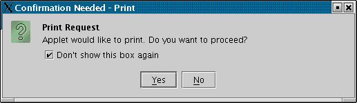
Fig. 11. Printer warning

To print a graph, click the "Print" button. The first time you do this, you will get a dialog box making sure that you indeed requested that something be sent to the printer (Fig. 11). Ths is a security measure in Java intended to handicap malicious code. Click "yes." A standard printing dialog box will appear. Proceed like you would with any other printing job. By default, the image will print in "landscape" (horizontal) layout. Due to Java security measures, changing the layout from the "properties" box in the print dialog box will not work. If you want to print in "portrait" (vertical), go to the Curve menu, select "Page Setup", and select "portrait".

Saving

To save the currently displayed graph to your computer, click the "save as" button. In the menu that will apper, select the file type you want, and adjust parameters such as image width, if desired. Press ok. If you have pop-up blocking software such as the google toolbar or a later version of IE browser, you may need to hold down the CTRL key while clicking the OK button.

Retrieving alignments

To view the underlying alignments for any curve, click on the curve to select it, then click the "Alignment" button. If you have pop-up blocking software (external, such as the google toolbar, or built-in, in IE 6 for example), you will need to disable it -- this is usually done by holding down the CTRL key while clicking the button. If you were looking at a region that contained only one alignment, it will be shown to you immediately. If there were several alignments in the region of interest, a window with details about each of the alignments will open, and you will need to select which one you want to look at. Each alignment that forms a given graph will be shown here, including the overlapped ones. You can get the alignments by clicking the appropriate links in the right-hand column.

Retrieving annotations

To get annotation for a given segment on the genome, click one of the curves to select it, then click the "I" button. If you have pop-up blocking software (external, such as the google toolbar, or built-in, in IE 6 for example), you will need to disable it -- this is usually done by holding down the CTRL key while clicking the button. A new browser window will open that shows details about the alignments in your region. Click the "Get Annotations in this region" link at the top to get a text file containing the annotation.

Retrieving sequences

To retrieve the sequences that were aligned to produce the curves you observe, click one of the curves to select it, then click the "I" button. If you have pop-up blocking software (external, such as the google toolbar, or built-in, in IE 6 for example), you will need to disable it -- this is usually done by holding down the CTRL key while clicking the button. A new browser window will open that shows details about the alignments in your region. The columns in the display you will see correspond to organisms involved in the alignment. Click on the "sequence" link to get that organism's sequence.

Submitting to rVISTA

To get transcription factor binding site predictions for a given alignment, click one of the curves to select it, then click the "I" button. If you have pop-up blocking software (external, such as the google toolbar, or built-in, in IE 6 for example), you will need to disable it -- this is usually done by holding down the CTRL key while clicking the button. A new browser window will open that shows details about the alignments in your region. Each alignment that forms a given graph will be shown here, including the overlapped ones. To submit the alignment to rVISTA, click on the "rVista" link in the left column. Note that rVISTA only takes one pairwise alignment as input, so if the region you are interested in is covered by several alignments, each one will need to be submitted separately.

Viewing in other Browsers

When another browser is available for the base genome, clicking the "browsers" button will open a new web browser window with the given section of the genome in this other browser. When multiple browsers are available, a choice of browsers will be presented. As usual, hold down the CTRL key when clicking on the button if you have a pop-up blocker.

Advanced

How to Change the Base Genome

When looking at an alignment of two organisms, it is sometimes useful to be able to change which organism is being used as the base. To do so, right-click on the curve you are interested in and select "Change Base Genome." If more than one region of the second organism was mapped to the region you are looking at, you will be presented with a choice of matches. Select the appropriate location and click "OK." If there is a one-to-one correspondence between the two regions, the browser will skip the menu and go straight to the correct location on the other organism.

How the Curve is Calculated

The Vista curve is calculated as a windowed-average identity score for the alignment. A variable sized window (Calc Window) is slid across the alignment and a score is calculated at each base in the coordinate sequence. That is, if the Calc Window is 100 base pairs, then the score for every point X is the percentage of exact matches between the two alignments in a 100bp-wide window centered on that point X. Due to resolution constraints when visualizing large alignments, it is often necessary to condense information about a hundred or more base-pairs into one display pixel. This is done by only graphing the maximal score of all the base pairs covered by that pixel.

Changing Curve Parameters

To adjust the parameters for a particular curve, click on it to select it and click the "Curve Parameters" button. A window with adjustable parameters will appear. You can adjust the following parameters:

• Calc Window: The size of the sliding window used to calculate conservation scores of each base pair which create theVISTA curve. Default is 100 base pairs.
• Min Cons Width: Minimum width a conserved region must be before it is painted as such. Default value is 100 base pairs.
• Cons Identity: Minumum percent conservation identity that must be maintained over the window ("min cons width") for a region to be considered conserved. Default value is 70%.
• Minimum and Maximum Y Lower and upper boundaries of the graph. Dropping the minimum Y value in areas of low conservation will allow you to see the these smaller peaks. Default value is 50% to 100%.
• Curve Name The label that is associated with the curve.

Changing the number of rows

To change the number of rows used to display the curves, use the "# Rows" drop-down menu in the left panel. The default is to automatically show as many rows as can fit on a single screen.

Changing the order of Curves

To change the order in which the curves are displayed on the browser, select the curve you want to move up or down and click the "Up/Down" buttons next to the curve name at the bottom of the screen.

Overlapping Contigs

When two or more data set contigs are aligned to the same region on the human genome, the Vista Genome Browser displays the maximum conservation for each pixel in the overlap region. The user can examine the contigs in the overlap individually by clicking the "Contig Details" button.

Coloring Rules

Conserved regions are defined as regions with conservation score of "Cons Identity" (75% by default) or higher, that are bigger than or equal to "Min Cons Width" (100 bp by default). Regions that satisfy this constraint are painted according to the annotation; all unannotated regions are painted as conserved non-coding regions (CNS).

Troubleshooting

Browser and Information buttons don't work

Usually this happens when a pop-up blocking software (external, such as the google toolbar, or built-in, in IE 6 for example) is enabled. To override the pop-up blocker, try holding down the CTRL key while clicking on the button you need.

Browser does not print in Opera

For some reason the default settings in the Opera browser do not grant Java applets printing priviliges. The easiest way to get around this is to save the picture you want as a PDF file and then print it from Acrobat Reader or your favorite PDF viewer. If you are so inclined, however, you can change the Opera configuration files to grant applets printing priviliges and never have to worry about this issue again:

1. Exit Opera Browser
2. Open the file C:\\Program Files\Opera7\classes\Opera.policy
3. After the line
   grant {
   add the following line:
   permission java.lang.RuntimePermission "queuePrintJob";
4. Save the file and launch Opera.